---
title: "Deconvolution Benchmark in Human DLPFC"
author: 
  - name: Louise Huuki-Myers
    affiliation:
    - &libd Lieber Institute for Brain Development, Johns Hopkins Medical Campus
    email: lahuuki@gmail.com
output: 
  BiocStyle::html_document:
    self_contained: yes
    toc: true
    toc_float: true
    toc_depth: 2
    code_folding: show
date: "`r doc_date()`"
package: "`r pkg_ver('DeconvoBuddies')`"
vignette: >
  %\VignetteIndexEntry{Deconvolution Benchmark in Human DLPFC}
  %\VignetteEncoding{UTF-8}  
  %\VignetteEngine{knitr::rmarkdown}
editor_options: 
  markdown: 
    wrap: 72
---

```{r setup, include = FALSE}
knitr::opts_chunk$set(
    collapse = TRUE,
    comment = "#>",
    crop = NULL ## Related to https://stat.ethz.ch/pipermail/bioc-devel/2020-April/016656.html
)
```

```{r vignetteSetup, echo=FALSE, message=FALSE, warning = FALSE}
## Bib setup
library("RefManageR")

## Write bibliography information
bib <- c(
    R = citation(),
    BiocStyle = citation("BiocStyle")[1],
    knitr = citation("knitr")[1],
    RefManageR = citation("RefManageR")[1],
    rmarkdown = citation("rmarkdown")[1],
    sessioninfo = citation("sessioninfo")[1],
    testthat = citation("testthat")[1],
    DeconvoBuddies = citation("DeconvoBuddies")[1]
)
```

# Introduction

## What is Deconvolution?

**Inferring the composition of different cell types in a bulk RNA-seq
data**

Deconvolution is a analysis that aims to calculate the proportion of
different cell types that make up a sample of bulk RNA-seq, based off of
cell type gene expression profiles in a single cell/nuclei RNA-seq
dataset.

<p align="center">

![Figure 1. Overview on how to use single cell data to infer the composition of bulk RNA-seq
samples](http://research.libd.org/DeconvoBuddies/reference/figures/Deconvolution.png)

</p>

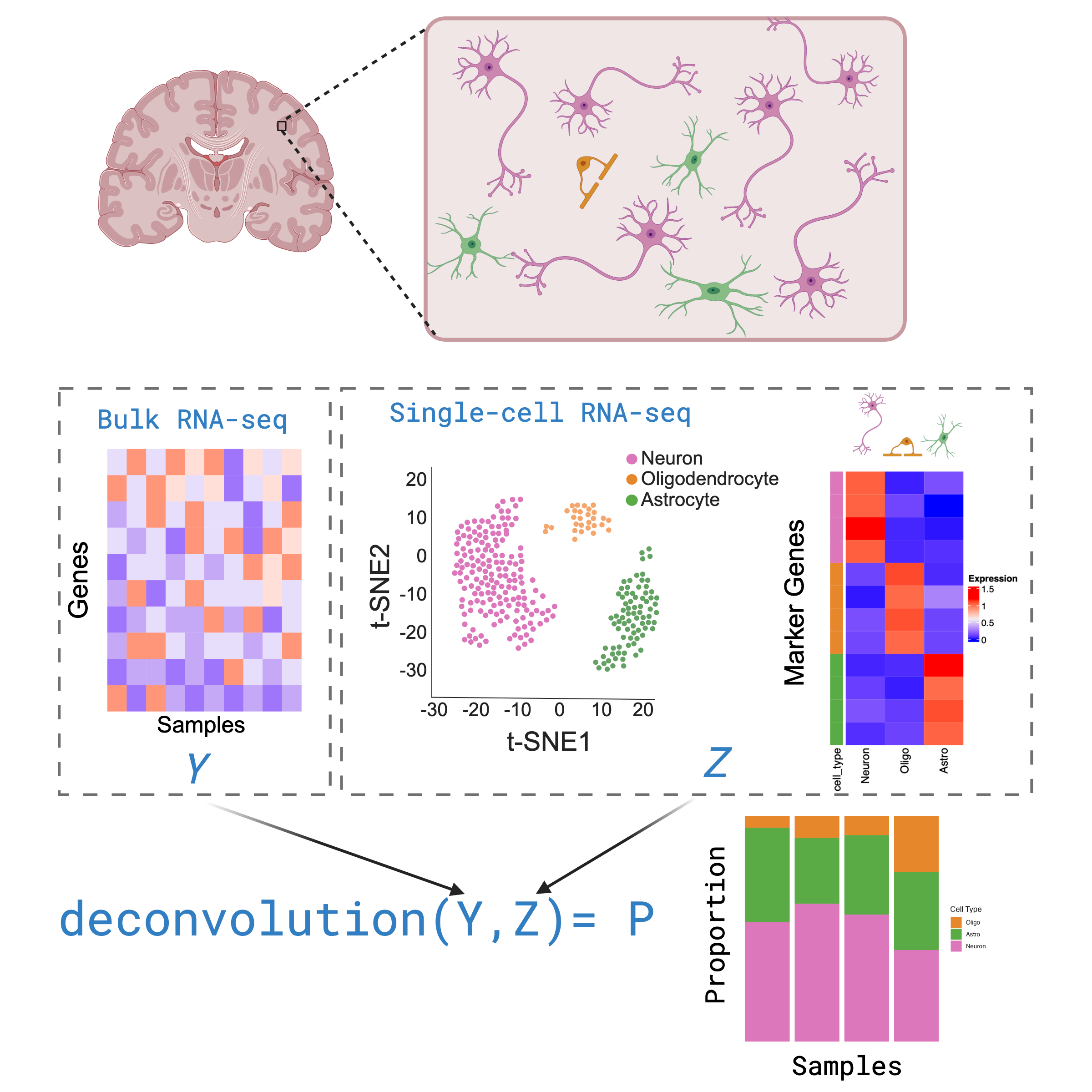
### Deconvolution Methods

There are 20+ published reference based deconvolution methods. Below are
a selection of 6 methods we tested in our [deconvolution benchmark
study](https://doi.org/10.1101/2024.02.09.579665).

| Approach                | Method     | Citation                                | Availability                                                              |
|-------------------|-----------------|-----------------|---------------------|
| weighted least squares  | DWLS       | Tsoucas et al, Nature Comm, 2019        | [R Package CRAN](https://cran.r-project.org/web/packages/DWLS/index.html) |
| Bias correction: Assay  | Bisque     | Jew et al, Nature Comm, 2020            | [R Package GitHub](https://github.com/cozygene/bisque)                                                          |
| Bias correction: Source | MuSiC      | Wang et al, Nature Communications, 2019 | [R Package GitHub](https://github.com/xuranw/MuSiC)                                                          |
| Machine Learning        | CIBERSORTx | Newman et al., Nature BioTech, 2019     | [Webtool](https://cibersortx.stanford.edu/)                               |
| Bayesian                | BayesPrism | Chu et al., Nature Cancer, 2022         | [Webtool/R Package](https://github.com/Danko-Lab/BayesPrism)              |
| linear                  | Hspe       | Hunt et al., Ann. Appl. Stat, 2021      | [R package GitHub](https://gjhunt.github.io/hspe/)                        |

## Goals of this Vignette

We will be demonstrating how to use `DeconvoBuddies` tools when applying
deconvolution with the `Bisque` package.

1.  Install and load required packages
2.  Download DLPFC RNA-seq data, and reference snRNA-seq data
3.  Find marker genes with `DeconvoBuddies` tools
4.  Run deconvolution with `BisqueRNA`
5.  Explore deconvolution output and create composition plots with
    `DeconvoBuddies` tools
6.  Check proportion against RNAScope estimated proportions

## Video Tutorial

Linked is a video from a presentation of an earlier version of this tutorial 
from our [LIBD Rstats club](https://research.libd.org/rstatsclub/). 

<iframe width="560" height="315" src="https://www.youtube.com/embed/6fTnp_hcYeI?si=UbkGNclU2q8I8WXO" title="YouTube video player" frameborder="0" allow="accelerometer; autoplay; clipboard-write; encrypted-media; gyroscope; picture-in-picture; web-share" referrerpolicy="strict-origin-when-cross-origin" allowfullscreen></iframe>

# Basics

# 1. Install and load required packages

`R` is an open-source statistical environment which can be easily
modified to enhance its functionality via packages.
`r Biocpkg("DeconvoBuddies")` is a `R` package available via the
[Bioconductor](http://bioconductor.org) repository for packages. `R` can
be installed on any operating system from
[CRAN](https://cran.r-project.org/) after which you can install
`r Biocpkg("DeconvoBuddies")` by using the following commands in your
`R` session:

## Install `DeconvoBuddies`

```{r "install", eval = FALSE}
if (!requireNamespace("BiocManager", quietly = TRUE)) {
    install.packages("BiocManager")
}

BiocManager::install("DeconvoBuddies")

## Check that you have a valid Bioconductor installation
BiocManager::valid()
```

## Load Other Packages

Let's load the packages we'll be using in this vignette.

```{r "load_packages", message=FALSE, warning=FALSE}
## Packages for different types of RNA-seq data structures in R
library("SummarizedExperiment")
library("SingleCellExperiment")
library("Biobase")

## For downloading data
library("spatialLIBD")

## Other helper packages for this vignette
library("dplyr")
library("tidyr")
library("tibble")
library("ggplot2")

## Our main package
library("DeconvoBuddies")
```

# 2. Download DLPFC RNA-seq data, and reference snRNA-seq data.

## Bulk RNA-seq data

Access the 110 sample Human DLPFC bulk RNA-seq dataset for LIBD described in more detail [here](https://github.com/LieberInstitute/Human_DLPFC_Deconvolution). These
samples\
are from 19 tissue blocks, and 10 neurotypical adult donors. Samples
were sequenced with two different `library_types` (polyA and
RiboZeroGold), and three different `RNA_extraction` (Cyto, Total, Nuc). There are in total n=110 samples after quality control.

```{r "load rse_gene"}
## use fetch deconvo data to load rse_gene
rse_gene <- fetch_deconvo_data("rse_gene")
rse_gene
# lobstr::obj_size(rse_gene)
# 41.16 MB

## Use gene "Symbol" as identifiers for the genes in rownames(rse_gene)
rownames(rse_gene) <- rowData(rse_gene)$Symbol

## bulk RNA seq samples were sequenced with different library types,
## and RNA extractions
table(rse_gene$library_type, rse_gene$library_prep)
```

## Reference snRNA-seq data

This data is paired with a single nucleus RNA-seq data set from
`spatialLIBD`. This dataset can be accessed with
`spatialLIBD::fetch_data()`.

```{r "load snRNA-seq"}
## Use spatialLIBD to fetch the snRNA-seq dataset used in this project
sce_path_zip <- fetch_deconvo_data("sce")

## unzip and load the data
sce_path <- unzip(sce_path_zip, exdir = tempdir())
sce <- HDF5Array::loadHDF5SummarizedExperiment(
    file.path(tempdir(), "sce_DLPFC_annotated")
)

# lobstr::obj_size(sce)
# 172.28 MB

## exclude Ambiguous cell type
sce <- sce[, sce$cellType_broad_hc != "Ambiguous"]
sce$cellType_broad_hc <- droplevels(sce$cellType_broad_hc)

## Check the number of genes by the number of nuclei that we
## have to work with:
dim(sce)

## Check the broad cell type distribution
table(sce$cellType_broad_hc)

## We're going to subset to the first 5k genes to save memory
## just for this example. You wouldn't do this on a full analysis.
sce <- sce[seq_len(5000), ]
```

## Orthogonal Cell Type Proportion from RNAScope/IF

An alternative method for calculating cell type proportions is through
imaging a slice of tissue with cell type probes using single molecule fluorescent _in situ_ hybridization (smFISH) experiments performed with RNAScope/IF (ImmunoFluorescence). Then
analyse the image to count cells and annotate them by cell type. In this
study we used [HALO from Indica Labs](https://indicalab.com/halo/) for this step.

The cell type proportions from the RNAScope/IF experiment will be used
to evaluate the accuracy of cell type proportion estimates.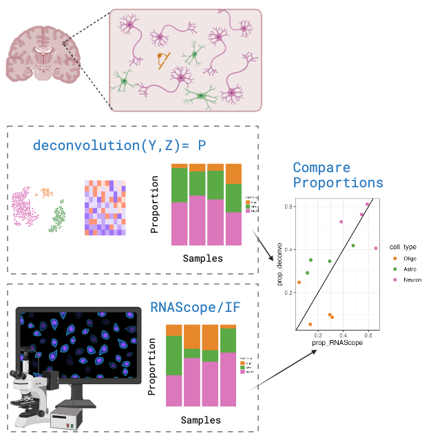

<p align="center">

![Figure 2. RNAScope/IF measures the cell type proportions through imaging](http://research.libd.org/DeconvoBuddies/reference/figures/Deconvolution_compare_proportions.png)

</p>


The RNAScope/IF proportion data is stored as a `data.frame` object in
`DeconvoBuddies::RNAScope_prop`.

Key columns in `RNAScope_prop`:

-   `SAMPLE_ID`: DLPFC Tissue block + RNAScope combination.

-   `Sample` : DLFPC Tissue block (Donor BrNum + DLPFC position).

-   `cell_type` : The cell type measured.

-   `n_cell` : the number of cells counted for the Sample and cell type.

-   `prop` : the calculated cell type proportion from n_cell

```{r "access RNAScope proportions"}
# Access the RNAScope proportion data.frame
data("RNAScope_prop")
head(RNAScope_prop)

## plot the RNAScope compositions
plot_composition_bar(
    prop_long = RNAScope_prop,
    sample_col = "SAMPLE_ID",
    x_col = "SAMPLE_ID",
    add_text = FALSE
) +
    facet_wrap(~Combo, nrow = 2, scales = "free_x")
```

Above we can see the cell proportions for each of the samples in either the `Circle` or the `Star` combination of RNAScope/IF probes. Each combination of RNAScope/IF probes was able to assess different sets of cell types. Two of them had to be used to measure the number of cell types studied in this case as there are limits on how many unique probes you can measure in a given RNAScope/IF experiment. For more details about the RNAScope/IF combinations, check the paper describing [this study](https://github.com/LieberInstitute/Human_DLPFC_Deconvolution).

# 3. Select Marker Genes

Marker genes are genes with high expression in one cell type and low
expression in other cell types, or "cell-type specific" expression.
These genes can be used to learn more about the identity and function of
cell types, but here we are interested in using a sets of cell type
specific marker genes to reduce noise in deconvolution and increase
accuracy.

We have developed a method for finding marker genes called the "Mean
Ratio". We calculate the *MeanRatio* for a target cell type for each
gene by dividing the mean expression of the target cell by the mean
expression of the next highest non-target cell type. Genes with the
highest *MeanRatio* values are selected as marker genes.

For a tutorial on marker gene selection check out  [Vignette: Finding Marker Genes with Deconvo Buddies](https://research.libd.org/DeconvoBuddies/articles/Marker_Finding.html).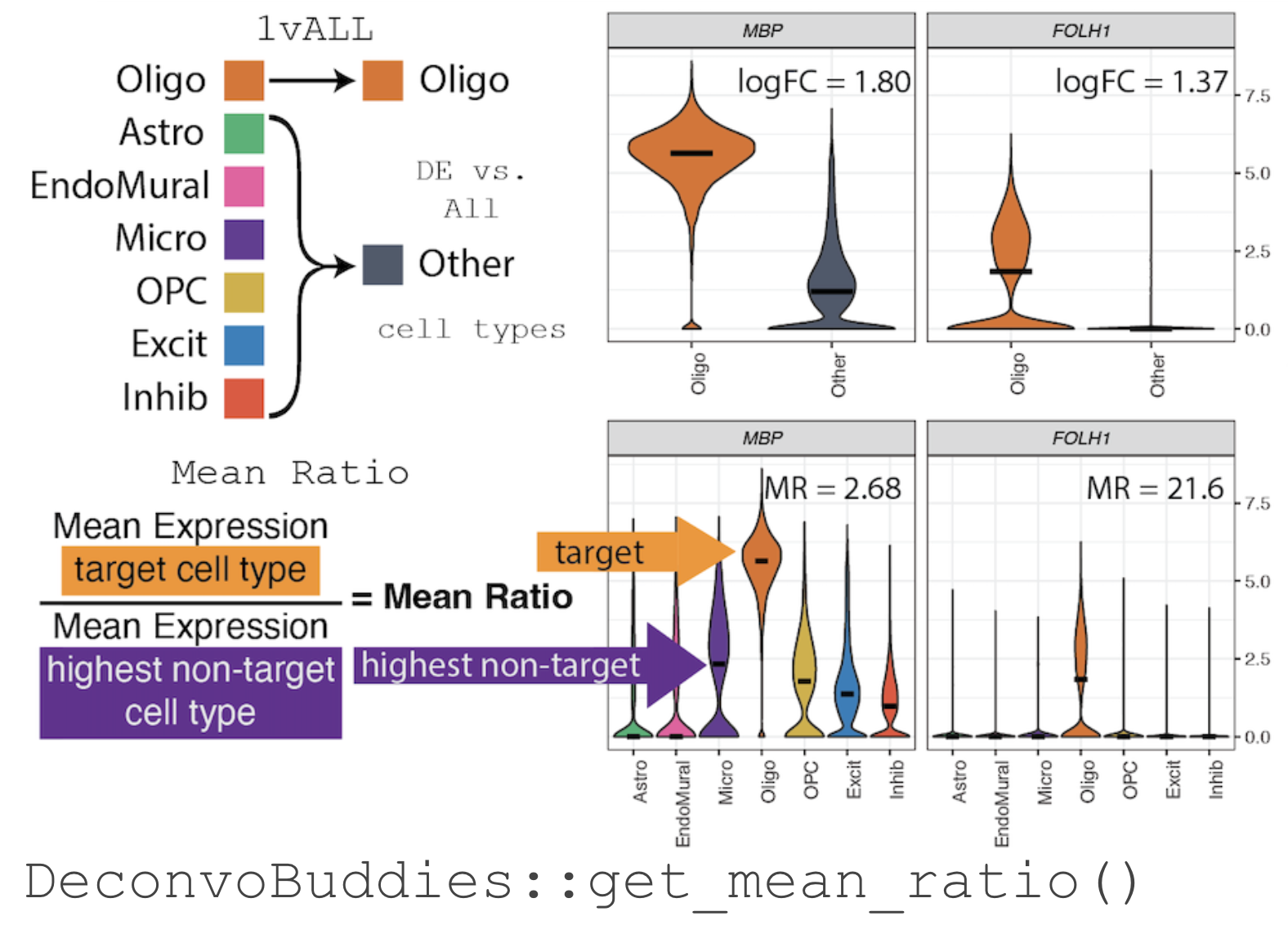

<p align="center">

![Figure 3. Mean Ratio calculation process compared to 1vALL Marker Gene
selection](http://research.libd.org/DeconvoBuddies/reference/figures/get_mean_ratio.png)

</p>

## Use `get_mean_ratio()` to find marker genes.

The function `DeconvoBuddies::get_mean_ratio()` calculates the
*MeanRatio* and the rank of genes for a specified cell type annotation
in an `SingleCellExperiment` object.

```{r "Run Mean Ratio"}
# calculate the Mean Ratio of genes for each cell type
marker_stats <- get_mean_ratio(sce,
    cellType_col = "cellType_broad_hc",
    gene_ensembl = "gene_id",
    gene_name = "gene_name"
)

# check the top gene ranked gene for each cell type
marker_stats |>
    group_by(cellType.target) |>
    slice(1)
```

The columns of this table are documented in detail at `DeconvoBuddies::get_mean_ratio()`. Though `cellType.target` lists the target cell type for which the *MeanRatio* is being calculated. It is the numerator of the *MeanRatio*. The `cellType.2nd` lists the cell type against which the target cell type is being compared. It is the denominator of the *MeanRatio*.

## Plot the top marker genes

Use `DeconvoBuddies` plotting tools to quickly plot the gene expression
of the top 4 Excitatory neuron marker genes across the
`cellType_broad_hc` cell type annotations.

```{r "plot marker genes"}
# plot expression across cell type the top 4 Excit marker genes
plot_marker_express(sce,
    stats = marker_stats,
    cell_type = "Excit",
    cellType_col = "cellType_broad_hc",
    rank_col = "MeanRatio.rank",
    anno_col = "MeanRatio.anno",
    gene_col = "gene"
)
```

Looks nice and cell type specific!

Note how `plot_marker_express()` lists the 2 cell types that are being compared that result in the specific numerical *MeanRatio* value being displayed. As we specified that our target cell type is `"Excit"` in our call to `plot_marker_express()`, the numerator is `Excit` in all the panels shown above.

### Create a List of Marker Genes

With the *MeanRatio* calculated, we will select the top 25 highest Mean
Ratio genes for each cell type, that also exists in the bulk data
`rse_gene`.

```{r "marker_list"}
# select top 25 marker genes for each cell type, that are also in rse_gene
marker_genes <- marker_stats |>
    filter(MeanRatio.rank <= 25 & gene %in% rownames(rse_gene))

# check how many genes for each cell type (some genes are not in both datasets)
marker_genes |> count(cellType.target)

# create a vector of marker genes to subset data before deconvolution
marker_genes <- marker_genes |> pull(gene)
```

# 4. Prep Data and Run Bisque

[*Bisque*](https://github.com/cozygene/bisque) is an R package for cell
type deconvolution. In our [deconvolution benchmark](https://github.com/LieberInstitute/Human_DLPFC_Deconvolution), we found it was a
top performing method. Below we will briefly show how to run `Bisque`'s
"reference based decomposition (deconvolution)".

## Prepare data

To run `Bisque` the snRNA-seq and bulk data must first be converted to
`Biobase::ExpressionSet()` format. We will subset our data to our selected
*MeanRatio* marker genes.

The snRNA-seq data must also be filtered for cells with no counts across
marker genes.

```{r "prep data as ExpressionSet"}
# NOT RUN - no longer running Bisque - see next section for details

if(FALSE){
## convert bulk data to Expression set, sub-setting to marker genes
## include sample ID
exp_set_bulk <- Biobase::ExpressionSet(
    assayData = assays(rse_gene[marker_genes, ])$counts,
    phenoData = AnnotatedDataFrame(
        as.data.frame(colData(rse_gene))[c("SAMPLE_ID")]
    )
)

## convert snRNA-seq data to Expression set, sub-setting to marker genes
## include cell type and donor information
exp_set_sce <- Biobase::ExpressionSet(
    assayData = as.matrix(assays(sce[marker_genes, ])$counts),
    phenoData = AnnotatedDataFrame(
        as.data.frame(colData(sce))[, c("cellType_broad_hc", "BrNum")]
    )
)

## check for nuclei with 0 marker expression
zero_cell_filter <- colSums(exprs(exp_set_sce)) != 0
message("Exclude ", sum(!zero_cell_filter), " cells")

exp_set_sce <- exp_set_sce[, zero_cell_filter]
}

```

## Run Bisque

`Bisque` needs the bulk and single cell `ExpressionSet` we prepared
above, plus columns in the single cell data that specify the cell type
annotation to use `cellType_broad_hc` and donor id (`BrNum` in this
data).

NOTE: Bisque is no longer available on CRAN (as of July 2025) so cannot be run in this vignette. 
We'll use pre-computed estimates for this vignette instead. (loaded in the next section).

```{r, "run Bisque"}
## NOT RUN - Bisque unavailable on CRAN

## Run Bisque with bulk and single cell ExpressionSet inputs
## For running deconvolution

# But the development version can be installed from github via:
# devtools::install_github("cozygene/bisque")

if(FALSE){
# library("BisqueRNA")

est_prop <- ReferenceBasedDecomposition(
    bulk.eset = exp_set_bulk,
    sc.eset = exp_set_sce,
    cell.types = "cellType_broad_hc",
    subject.names = "BrNum",
    use.overlap = FALSE
)

## Examine the output from Bisque, transpose to make it easier to work with
est_prop <- t(est_prop$bulk.props)

}

```

## Explore Output

`Bisque` predicts the proportion of the cell types in `cellType_broad_hc`
for each sample in the bulk data.

```{r, "deconvo output"}
## Load the pre-computed estimated proportions
data("est_prop")

## sample x cell type matrix
head(est_prop)
```

# 5. Explore deconvolution output and create composition plots with `DeconvoBuddies` tools

To visualize the cell type proportion predictions, we can plot cell type
composition bar plots with `DeconvoBuddies::plot_composition_bar()`,
either the prediction for each sample, or the average proportion over a
group of samples.

```{r, "composition plots"}
## add Phenotype data to proportion estimates
pd <- colData(rse_gene) |>
    as.data.frame() |>
    select(SAMPLE_ID, Sample, library_combo)

## make proportion estimates long so they are ggplot2 friendly
prop_long <- est_prop |>
    as.data.frame() |>
    tibble::rownames_to_column("SAMPLE_ID") |>
    tidyr::pivot_longer(!SAMPLE_ID, names_to = "cell_type", values_to = "prop") |>
    left_join(pd)

## create composition bar plots

## for all library preparations by sample n=110
## Remove the SAMPLE_ID names since they are very long using ggplot2::theme()
plot_composition_bar(
    prop_long = prop_long,
    sample_col = "SAMPLE_ID",
    x_col = "SAMPLE_ID",
    add_text = FALSE
) +
    theme(axis.text.x = element_blank(), axis.ticks.x = element_blank())

## Average by brain donor
plot_composition_bar(
    prop_long = prop_long,
    sample_col = "SAMPLE_ID",
    x_col = "Sample",
    add_text = FALSE
)

## Each brain donor has up to 6 unique RNA library type and RNA extraction
## combinations
table(prop_long$Sample) / length(unique(prop_long$cell_type))

## Here are the 6 "SAMPLE_ID" values for brain donor with ID "Br8667_mid"
unique(prop_long$SAMPLE_ID[prop_long$Sample == "Br8667_mid"])
```

This is a more complex scenario than the one from the [introductory vignette](https://research.libd.org/DeconvoBuddies/articles/DeconvoBuddies.html) where we were using random data. The first plot shows each of the n=110 bulk RNA-seq samples we have. The second plot shows the composition using the average across the 6 RNA library types and RNA extractions for each brain donor. 

# 6. Check proportion against RNAScope/IF estimated proportions

Note to compare the deconvolution results to the RNAScope/IF proportions,
Oligo and OPC need to be added together.

```{r "compare prop"}
## Combine Oligo and OPC into OligoOPC
prop_long_opc <- prop_long |>
    mutate(cell_type = gsub("Oligo|OPC", "OligoOPC", cell_type)) |>
    group_by(SAMPLE_ID, Sample, library_combo, cell_type) |>
    summarize(prop = sum(prop)) |>
    ungroup()

prop_long_opc |> count(cell_type)

## Join RNAScope/IF and Bisque cell type proportions
prop_compare <- prop_long_opc |>
    inner_join(
        RNAScope_prop |>
            select(Sample, cell_type, prop_RNAScope = prop, prop_sn),
        by = c("Sample", "cell_type")
    )
```

We can now calculate the correlation plot a scatter plot of the proportions. Note that you can change the type of correlation algorithm used in the `cor()` function. The default method is `"pearson"`.

```{r "proportion scatter"}
## compute correlation with RNAScope/IF proportions
cor(prop_compare$prop, prop_compare$prop_RNAScope)

## Scatter plot with RNAScope/IF proportions
prop_compare |>
    ggplot(aes(x = prop_RNAScope, y = prop, color = cell_type, shape = library_combo)) +
    geom_point() +
    geom_abline()


## correlation with snRNA-seq proportion
cor(prop_compare$prop, prop_compare$prop_sn)

## Scatter plot with RNAScope/IF proportions
prop_compare |>
    ggplot(aes(x = prop_sn, y = prop, color = cell_type, shape = library_combo)) +
    geom_point() +
    geom_abline()
```

In the first plot we can see how `Bisque` overestimates the proportion of excitatory neurons (`Excit`) when compared against RNAScope/IF as all `Excit` points are higher than the diagonal line shown in black. 

In the second plot we can see how `Bisque` proportions are closer to the snRNA-seq proportions. After all, given the [challenges in generating orthogonal cell type proportion data](https://doi.org/10.1186/s13059-023-03123-4), `Bisque` and other deconvolution methods were developed by comparing against simulated data, sometimes using pseudo-bulk sc/snRNA-seq data.

# 7. How to run deconvolution with `hspe`

*hspe* (formerly called *dtangle*) is another R package for deconvolution. It
was also a top performing method in our [deconvolution benchmark](https://github.com/LieberInstitute/Human_DLPFC_Deconvolution).

`hspe` is [downloadable](https://gjhunt.github.io/hspe/) from GitHub but
can't be shown on this vignette as Bioconductor packages cannot use packages from GitHub.

Below we show some example code to prepare input data and run `hspe` (not run
here):

```{r "prep and run hspe"}
if (FALSE) {
    ## Install hspe
    # if (!requireNamespace("hspe", quietly = TRUE)) {
    #     ## Install version 0.1 which is the one listed on the main documentation
    #     ## at https://github.com/gjhunt/hspe/tree/main?tab=readme-ov-file#software
    #     remotes::install_url("https://github.com/gjhunt/hspe/raw/main/hspe_0.1.tar.gz")
    #     ## Alternatively, install from the latest version on GitHub with:
    #     # remotes::install_github("gjhunt/hspe", subdir = "lib_hspe")
    #
    #     ## As of 2024-08-23, it's been 3 years since files were last modified
    #     ## at https://github.com/gjhunt/hspe/tree/main/lib_hspe.
    # }
    # library("hspe")

    # pseudobulk the sce data by sample + cell type
    sce_pb <- spatialLIBD::registration_pseudobulk(sce,
        var_registration = "cellType_broad_hc",
        var_sample_id = "Sample"
    )


    ## extract the gene expression from the bulk rse_gene
    mixture_samples <- t(assays(rse_gene)$logcounts)
    mixture_samples[1:5, 1:5]

    ## create a vector of indexes of the different cell types
    pure_samples <- rafalib::splitit(sce_pb$cellType_broad_hc)

    ## extract the the pseudobulked logcounts
    reference_samples <- t(assays(sce_pb)$logcounts)
    reference_samples[1:5, 1:5]

    ## check the number of genes match in the bulk (mixture) and single cell (reference)
    ncol(mixture_samples) == ncol(reference_samples)

    ## run hspe
    est_prop_hspe <- hspe(
        Y = mixture_samples,
        reference = reference_samples,
        pure_samples = pure_samples,
        markers = marker_genes,
        seed = 10524
    )
}
```

# Conclusion

In this vignette we have demonstrated some of the functions and data in
the `DeconvoBuddies` package, and how to use them in a deconvolution
workflow to predict cell type proportions. We used real data from a study
on [human brain](https://github.com/LieberInstitute/Human_DLPFC_Deconvolution).

# Reproducibility

The `r Biocpkg("DeconvoBuddies")` package
`r Citep(bib[["DeconvoBuddies"]])` was made possible thanks to:

-   R `r Citep(bib[["R"]])`
-   `r Biocpkg("BiocStyle")` `r Citep(bib[["BiocStyle"]])`
-   `r CRANpkg("knitr")` `r Citep(bib[["knitr"]])`
-   `r CRANpkg("RefManageR")` `r Citep(bib[["RefManageR"]])`
-   `r CRANpkg("rmarkdown")` `r Citep(bib[["rmarkdown"]])`
-   `r CRANpkg("sessioninfo")` `r Citep(bib[["sessioninfo"]])`
-   `r CRANpkg("testthat")` `r Citep(bib[["testthat"]])`

This package was developed using `r BiocStyle::Biocpkg("biocthis")`.

`R` session information.

```{r reproduce3, echo=FALSE}
## Session info
library("sessioninfo")
options(width = 120)
session_info()
```

# Bibliography

This vignette was generated using `r Biocpkg("BiocStyle")`
`r Citep(bib[["BiocStyle"]])` with `r CRANpkg("knitr")`
`r Citep(bib[["knitr"]])` and `r CRANpkg("rmarkdown")`
`r Citep(bib[["rmarkdown"]])` running behind the scenes.

Citations made with `r CRANpkg("RefManageR")`
`r Citep(bib[["RefManageR"]])`.

```{r vignetteBiblio, results = "asis", echo = FALSE, warning = FALSE, message = FALSE}
## Print bibliography
PrintBibliography(bib, .opts = list(hyperlink = "to.doc", style = "html"))
```